
Study Design#
Overall Study Design for National Databases#
The Graph below recaps the overall study design for Aims 1-2
Show code cell source
import networkx as nx
import matplotlib.pyplot as plt

G = nx.DiGraph()
G.add_node("OPTN", pos=(-4000, 800))
G.add_node("NHANES", pos=(-4000, 0))
G.add_node("Scenarios", pos=(-4000, -800))
G.add_node("CMS", pos=(0, 400))
G.add_node("NDI", pos=(0, -400))
G.add_node("ESRD", pos=(4000, 400))
G.add_node("Death", pos=(4000, -400))

G.add_edges_from([("OPTN", "CMS"), ("OPTN", "NDI")])
G.add_edges_from([("NHANES", "CMS"), ("NHANES", "NDI"), ("Scenarios", "NHANES")])
G.add_edges_from([("CMS", "ESRD"), ("NDI", "Death")])

pos = nx.get_node_attributes(G, 'pos')
labels = {"OPTN": "OPTN\n(Donors)",
          "NHANES": "NHANES\n(Nondonors)",
          "Scenarios": "Scenarios\n(Personalized)",
          "CMS": "CMS",
          "NDI": "NDI",
          "ESRD": "ESRD",
          "Death": "Death"}

# Update color for the "Scenarios" node
node_colors = ["lavender", "lavender", "lightblue", "lightgreen", "lightgreen", "lightpink", "lightpink"]

edge_styles = [("NHANES", "Scenarios", "dashed")]

plt.figure(figsize=(8, 8))
nx.draw(G, pos, with_labels=False, node_size=15000, node_color=node_colors, linewidths=2, edge_color='black', style='solid')
nx.draw_networkx_labels(G, pos, labels, font_size=10, font_weight='bold')
nx.draw_networkx_edges(G, pos, edgelist=edge_styles, edge_color='black', style='dashed', width=3)
plt.xlim(-5000, 5000)
plt.ylim(-1000, 1000)
plt.axis("off")
plt.show()
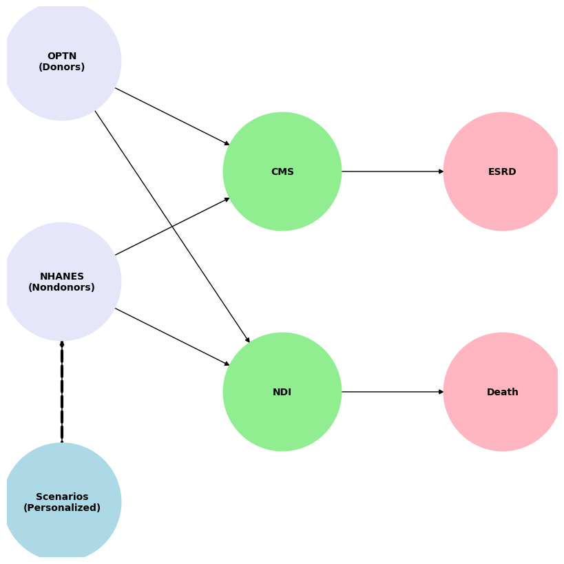

Fig. 3 Using data from the Scientific Registry of Transplant Recipients from 1988 to 2020, we estimated perioperative mortality (death within 90 days of donation), 30-year mortality, and risk of ESRD. Death events were captured through the Organ Procurement and Transplantation Network (OPTN) living donor follow-up reported by transplant programs, the National Technical Information Service Limited Access Death Master File, and deaths made available to the OPTN contractor through an interagency data-sharing agreement between the Centers for Medicare & Medicaid Services (CMS) and the Health Resources and Services Administration. These were secondarily verified by the OPTN contractor. Per OPTN policy, all donor deaths within two years of donation must be reported within 72 hours of the hospital becoming aware of the death. ESRD development was ascertained using Centers for Medicare & Medicaid Services data and defined as the initiation of maintenance dialysis, placement on the transplant waiting list, or receipt of a living or deceased donor kidney transplant, whichever occurred first. The healthy nondonor control population was derived from a cohort of 73,000 participants in the third National Health and Nutrition Examination Survey (NHANES). The National Center for Health Statistics performed linkages to the CMS and National Death Index to to ascertain ESRD and death. Both national datasets provided robust comparisons of donor and nondonor risks.#
Personalized Scenarios for Healthy Nondonor Candidates#
Personalized Risk Model Description#
The app employs a personalized risk model based on the survival function:
This equation calculates the cumulative probability of an event (e.g., end-stage renal disease, mortality, or hospitalization) over a specified follow-up period. The components of the model are as follows:
1. Baseline Hazard Function: \( h_0(t) \)#
The baseline hazard function, \( h_0(t) \), represents the risk of the event occurring for a reference population (base-case) at any given time \( t \).
It is nonparametric, meaning it does not assume a specific mathematical form but is instead estimated directly from the data.
This serves as the foundational risk profile to which adjustments for individual characteristics are applied.
2. Risk Adjustment: \( \text{exp}(X\beta) \)#
The term \( \text{exp}(X\beta) \) is a scaling factor derived from a maximum-likelihood estimate of the relative hazard for a specific individual compared to the base-case.
It accounts for differences in risk due to explanatory variables \( X \), such as:
Demographics: Age, sex, race/ethnicity.
Clinical Characteristics: Blood pressure, kidney function (e.g., GFR, albumin levels), or comorbidities (e.g., diabetes, hypertension).
Lifestyle Factors: Smoking status, physical activity levels.
\( \beta \) represents the regression coefficients that quantify the log-scale relationship between the explanatory variables and the hazard.
3. Follow-Up Period: \( t \)#
\( t \) is the time horizon over which risk is assessed. For example:
Currently, the app considers 30 years of follow-up for nondonors and 15 years of follow-up for donors. With our established infrastructure, updating this to 30 years of follow-up for donors should take no more than a day (the script has to be run remotely at SRTR)
The app also considers 90 day mortality in the perioperative period
How It Works#
The app calculates the cumulative hazard by integrating the adjusted hazard function over time:
This cumulative hazard reflects the total “exposure” to risk over the follow-up period.
The survival probability is then derived using the exponential function \( e^{-\int h_0(t) \, \text{exp}(X\beta) \, dt} \), representing the likelihood that the event has not occurred by time \( t \).
Finally, the personalized risk is calculated as:
This value indicates the cumulative probability of the event occurring by a given time point.
Advantages of the Model#
Personalization: By incorporating individual-level explanatory variables \( X \), the app generates a risk estimate tailored to each user’s unique clinical profile.
Flexibility: The nonparametric baseline hazard \( h_0(t) \) allows the model to adapt to observed patterns in the data without restrictive assumptions.
Transparency: Users can explore how changes in \( X \) (e.g., improving blood pressure or quitting smoking) affect their personalized risk.
Future Enhancements#
Extended Follow-Up: Incorporating longer follow-up periods (e.g., 30 years) will improve the model’s utility for younger individuals or even older individuals with up 30 years of residual life expectancy.
Dynamic Risk Updating: Incorporating real-time updates to \( X \) as users input new clinical or lifestyle data, enabling iterative risk recalibration.
Interactive Visualizations: Presenting the risk curve for donors alongside the one for controls offers what Locke described in her editorial as the “idea”. 5. Furthermore, our inclusion of 90% confidence intervals allows more advanced users to consider the error of margin in their inferences.